Getting Familiar with the DHQ Article and Citation Data
library(tidyverse)
## Loading tidyverse: ggplot2
## Loading tidyverse: tibble
## Loading tidyverse: tidyr
## Loading tidyverse: readr
## Loading tidyverse: purrr
## Loading tidyverse: dplyr

## Conflicts with tidy packages ----------------------------------------------

## filter(): dplyr, stats
## lag():    dplyr, stats
(Reading In) The Data
The data I’ll be working with this semester in Ryan Cordell’s Humanities Data Analysis graduate course is provided by Digital Humanities Quarterly, the leading open-access journal of digital humanities: these consist of ~180 of the 250+ articles published since its founding in 2007, up to 2014. The corpus contains the full content of each of these XML-encoded articles. Each encoded article contains a header with extensive metadata, including publication and some author information, most notably their university affiliation. Also included is an XML-based bibliographic database, which aggregates the bibliographic information from the backmatter of each encoded article.
For the purposes of this post, I will be making exclusive use of aggregate article and citation data assembled by the journal from the article corpus using XSLT stylesheets. The data are read in from two provided tsv files, each into its own tibble: one tibble contains information about the DHQ articles themselves, and the other contains information about the works that are cited in those articles.
## Parsed with column specification:
## cols(
##   `article id` = col_integer(),
##   author = col_character(),
##   year = col_integer(),
##   title = col_character(),
##   `journal/conference/collection` = col_character(),
##   abstract = col_character(),
##   `reference IDs` = col_character(),
##   isDHQ = col_integer()
## )

## Parsed with column specification:
## cols(
##   `article id` = col_character(),
##   author = col_character(),
##   year = col_character(),
##   title = col_character(),
##   `journal/conference/collection` = col_character(),
##   abstract = col_character(),
##   `reference IDs` = col_character(),
##   isDHQ = col_integer()
## )

## Warning in eval(substitute(expr), envir, enclos): NAs introduced by
## coercion
Both take on the same form and have the same 8 variables. Each observation is a single work, which is represented by a unique identifier in the article id variable. Other variables that are populated in both datasets include author, title, and year published; what journal/conference/collection the work is from; and a discrete variable isDHQ that marks whether or not the work is a DHQ article. This last variable uses 0=False and 1=True, so it’s been coerced to a boolean variable.
union(names(dhq_articles),names(dhq_citations))
## [1] "article id"                    "author"
## [3] "year"                          "title"
## [5] "journal/conference/collection" "abstract"
## [7] "reference IDs"                 "isDHQ"
Abstracts are available for the DHQ articles but not the cited works, since the cited works are not maintained by DHQ.
str(dhq_articles$abstract)
## chr [1:178] "A review of Willard McCarty's Humanities Computing." ...
str(dhq_citations$abstract)
## chr [1:3821] NA NA NA NA NA NA NA NA NA NA NA ...
The main mechanism for linking articles with their cited works is in the reference IDs variable: the observation for each DHQ article lists the IDs associated with the works cited in that article, separated by pipe characters. This is not true for the cited works, since the materials cited by cited works are not necessarily hosted by DHQ, and are thus not tracked.
str(dhq_articles$`reference IDs`)
## chr [1:178] "hockey2000 | mcgann2001a | sutherland1997 | schreibman2004" ...
str(dhq_citations$`reference IDs`)
## chr [1:3821] NA NA NA NA NA NA NA NA NA NA NA ...
All of the 178 DHQ articles in the corpus are appropriately marked as being DHQ articles in the relevant variables.
dhq_articles %>%
  count(isDHQ)
## # A tibble: 1 × 2
##   isDHQ     n
##   <lgl> <int>
## 1  TRUE   178
dhq_citations %>%
  group_by(isDHQ)%>%
  summarize(count=n())
## # A tibble: 2 × 2
##   isDHQ count
##   <lgl> <int>
## 1 FALSE  3790
## 2  TRUE    31
dhq_citations %>%
  filter(isDHQ == TRUE) %>%
  group_by(`journal/conference/collection`) %>%
  summarize(count=n())
## # A tibble: 1 × 2
##   `journal/conference/collection` count
##                             <chr> <int>
## 1    Digital Humanities Quarterly    31
A note: What may not be apparent in my “finished” post is that this exploratory analysis, in the sense that Grolemund and Wickham use the term in R for Data Science, helped me to find missing delimiters in the tsv file of citations: coerced NAs were emerging in the isDHQ count because the information for that variable was stored in another for a couple of records (see my commented out notes when reading in the .tsv files). I decided to continue on with those observations as NAs in the interim, but another flag that there was an issue with the data was thrown up when I tried to pose another question to it: when I tried finding the most-cited work, which I do later in the notebook, I was unable to locate that citation in the citation tibble from the reference ID yielded by transformation of the article tibble. This is because the issue propagated, causing large swatches of observations to be left out of that dataframe, rather than affecting only the observations on the mal-formed lines.
Fixing the erroneous observations visibly changed the results of the analysis. Even at this early stage, throwing research questions at the data, and transforming it to answer those questions, helped to investigate the quality of that data and clean it (I am comfortable using the word “clean” here despite Rawson and Muñoz’s critique of the term, since fixing missing delimiters to standardize the data according to what it was intended to be structured like in the first place is, I would argue, less value-laden than the types of cleaning they target–it is not imposing a new standardization.) That said, I am currently leaving out two observations because I can’t yet figure out why they can’t be parsed; so, there are two cited works absent from the following analysis in its current form.
Preliminary Analysis
Articles over Time
We might be interested in visualizing how many articles were published each year over the journal’s history.
dhq_articles %>%
  group_by(year) %>%
  summarize(count = n()) %>%
  ggplot(aes(x = year, y = count)) +
  geom_point() +
  geom_smooth() +
  ggtitle("Articles Published over DHQ Lifetime")
## `geom_smooth()` using method = 'loess'

## Warning: Removed 1 rows containing non-finite values (stat_smooth).

## Warning: Removed 1 rows containing missing values (geom_point).
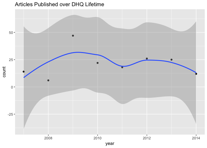
It looks like there was a small spike in articles published in the journal’s third year of publication. It may be of interest to aggregate the volume and issue metadata encoded in each article to make the temporal data more granular. We could then additionally isolate issues–say, special issues.
From when are works cited in DHQ articles?
Perhaps we’re interested in plotting the publication dates of the cited works instead of the articles. From when are DHQ authors citing?
dhq_citations %>%
  group_by(year) %>%
  summarize(count = n()) %>%
  ggplot() + aes(x = year, y=count) +
  geom_point() +
  ggtitle("Publication Dates of Materials Cited in DHQ Articles")
## Warning: Removed 1 rows containing missing values (geom_point).
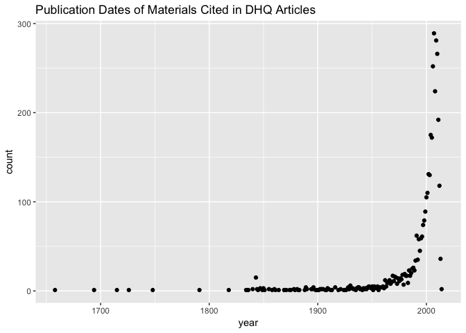
Most of the material cited by DHQ authors is written after the late 20th century, which makes sense for a journal of digital humanities. It may be of interest to plot the publication dates of cited materials versus the article publication dates to get an overview of when folks were citing from at their time of writing. This is one example of an analysis that would rely on linking the DHQ articles to their cited materials using the reference IDs–a comparitively challenging task. This would allow us, however, to ask more targeted questions of this citation date distribution. Are materials from certain eras–contemporary, recent past, before mid-century–being cited in the same articles, or by the same sets of authors?
In the mean time, we might look to the left extreme of the plot of the data we already have: are the oldest sources being cited?
dhq_citations %>%
  group_by(year) %>%
  select(year,author,title) %>%
  arrange(year)
## Source: local data frame [3,821 x 3]
## Groups: year [147]
##
##     year               author
##    <int>                <chr>
## 1   1658       Newman, Samuel
## 2   1694      Addison, Joseph
## 3   1715      Pope, Alexander
## 4   1726      Swift, Jonathan
## 5   1748          Hume, David
## 6   1791       Boswell, James
## 7   1818         Austen, Jane
## 8   1834            Hicks, E.
## 9   1835 Hawthorne, Nathaniel
## 10  1836 Hawthorne, Nathaniel
## # ... with 3,811 more rows, and 1 more variables: title <chr>
It appears that many of the older sources are primary or literary texts. While it isn’t included in the aggregate data, the dataset does contain encoded information about the genre of cited sources. This information is limited, however, to whether the source was a book, journal article, website, &c; it says nothing about whether e.g. the books cited were primary or secondary sources. This is a limitation of the current dataset, since it would be of particular interest for our purposes to be able to isolate authors’ engagement with academic conversations, who are citing monographs in addition to journal articles. Encoding at this level is beyond the scope of DHQ’s editorial staff, since they would have to research materials cited in the articles they have accepted and are encoding. Conversely, author-reported information would introduce its own editorial challenges.
Independently coding for this as a researcher would elicit non-trivial issues of labor (it takes a while) and taxonomy (is the same source “primary” or “secondary” always for the purposes of a DHQ article, or does it depend on its context?). Still, incorporating the citation genre information DHQ has already encoded may be useful, since we can then isolate at least the journal articles that DHQ authors are citing and plot when they are from. And since the number of articles is less than the number of citations, a slightly more achieveable goal might be to focus on the articles (rather than the cited works) and code whether each DHQ article is a book or collection review, literature review, argument-driven piece, etc. Are DHers citing primarily older conversations (building on or responding to previous expertise) or are they citing conversations contemporary to them? In what types of articles are they doing each?
Speaking of, let’s zoom in on the period after 2007, when DHQ came into being, and see how many of the cited materials in that period are DHQ articles. Here’s a plot of the raw citation count:
dhq_citations %>%
  group_by(year,isDHQ) %>%
  summarize(count=n()) %>%
  filter(year>=2007, isDHQ == TRUE) %>%
  ggplot() + aes(x = year, y = count) +
  geom_point() +
  ggtitle("Citations of DHQ Articles in other DHQ Articles, by Year")
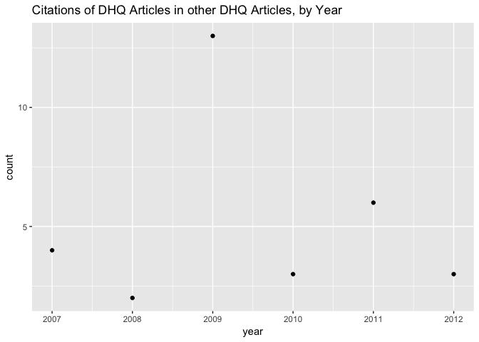
It would be more informative for the vertical axis to be a percentage of the total publication count for each year than as raw frequencies.
dhq_citations %>%
  filter(year >= 2007) %>%
  group_by(year) %>%
  mutate(total_year_pub=n()) %>%
  select(isDHQ, year, total_year_pub) %>%
  group_by(year,isDHQ, total_year_pub) %>%
  summarize(count = n()) %>%
  mutate(percentage = (count/total_year_pub)*100) %>%
  ggplot() + aes(x = year, y = percentage, color=isDHQ) +
  geom_point() +
  geom_text(aes(label=round(percentage,1)),hjust=0, vjust=0) +
  ggtitle("Percentage of DHQ Citations that are other DHQ Articles, by Year")
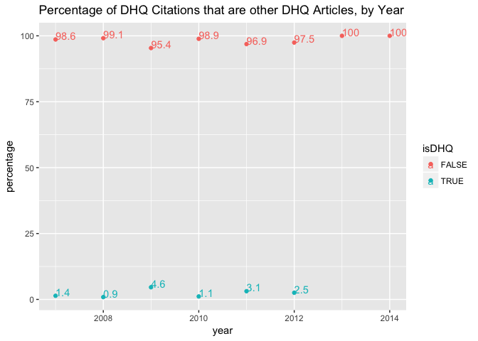
A relatively small percentage of citations in DHQ are internal citations of other DHQ articles. This seems sensible. The journal’s third year of publication, 2009, is again a spike: perhaps there was a special issue in that year that incouraged extensive intra-journal communication? That would explain the increase in number of articles published as well as the high percentage of internal citations. On the whole, perhaps the percentages are actually even high. We might want to compare across journals for reference.
It may be of more interest to look at how many articles contain any citation of a DHQ article; this might be a more measure of the degree of intrajournal collaboration. This task, like the article and citation year problem described above, however, is more challenging: it also involves combining data from the two tibbles.
What works are cited in DHQ articles?
Let’s start looking at the identities of the cited works and obtain a list of the works most frequently cited in DHQ.
A technical note: Because the number of reference IDs separated by pipe characters, and thereby how many columns we need, varies; using tidyr::separate for this seems challenging. We could probably have used tidyr::separate in combination with its fill argument, if we knew the greatest number of citations a single article has. Instead, we can use the strsplit function to add a new variable that contains a combined list containing the reference ids for each observation. Then, we unnest this list: the effect is that a new observation was created for every reference ID with the corresponding article ID. Upon grouping by article ID, we can define a new variable tracking the row number of the reference ID within each article ID. tidyr::spread can then be used to make a wide tibble, from which grouping and the no longer relevant reference IDs column are removed. The result is a wide tibble in which each observation is an article with its associated ID, and numbered variables containing each reference ID.
citation_ids_expanded <- dhq_articles %>%
  mutate(list = strsplit(`reference IDs`,"\\|"))  %>%
  unnest(list) %>%
  group_by(`article id`)  %>%
  mutate(row = row_number()) %>%
  spread(row, list)  %>%
  group_by()


citation_ids_expanded %>%
    select(-(author:isDHQ))
## # A tibble: 178 × 131
##    `article id`           `1`           `2`              `3`
## *         <int>         <chr>         <chr>            <chr>
## 1             1   hockey2000   mcgann2001a   sutherland1997
## 2             2  aarseth1997   aarseth2000      aarseth2004
## 3             3    about2006    about2006a        ayers1999
## 4             4 anderson2003       bia2003      chilton2006
## 5             5  benabou1987      bens1980      bergens1999
## 6             6          <NA>          <NA>             <NA>
## 7             7          <NA>          <NA>             <NA>
## 8             8          <NA>          <NA>             <NA>
## 9             9  aarseth1997   aarseth2001       adams2007c
## 10           10 anderson2006     bates1997         berg2004
## # ... with 168 more rows, and 127 more variables: `4` <chr>, `5` <chr>,
## #   `6` <chr>, `7` <chr>, `8` <chr>, `9` <chr>, `10` <chr>, `11` <chr>,
## #   `12` <chr>, `13` <chr>, `14` <chr>, `15` <chr>, `16` <chr>,
## #   `17` <chr>, `18` <chr>, `19` <chr>, `20` <chr>, `21` <chr>,
## #   `22` <chr>, `23` <chr>, `24` <chr>, `25` <chr>, `26` <chr>,
## #   `27` <chr>, `28` <chr>, `29` <chr>, `30` <chr>, `31` <chr>,
## #   `32` <chr>, `33` <chr>, `34` <chr>, `35` <chr>, `36` <chr>,
## #   `37` <chr>, `38` <chr>, `39` <chr>, `40` <chr>, `41` <chr>,
## #   `42` <chr>, `43` <chr>, `44` <chr>, `45` <chr>, `46` <chr>,
## #   `47` <chr>, `48` <chr>, `49` <chr>, `50` <chr>, `51` <chr>,
## #   `52` <chr>, `53` <chr>, `54` <chr>, `55` <chr>, `56` <chr>,
## #   `57` <chr>, `58` <chr>, `59` <chr>, `60` <chr>, `61` <chr>,
## #   `62` <chr>, `63` <chr>, `64` <chr>, `65` <chr>, `66` <chr>,
## #   `67` <chr>, `68` <chr>, `69` <chr>, `70` <chr>, `71` <chr>,
## #   `72` <chr>, `73` <chr>, `74` <chr>, `75` <chr>, `76` <chr>,
## #   `77` <chr>, `78` <chr>, `79` <chr>, `80` <chr>, `81` <chr>,
## #   `82` <chr>, `83` <chr>, `84` <chr>, `85` <chr>, `86` <chr>,
## #   `87` <chr>, `88` <chr>, `89` <chr>, `90` <chr>, `91` <chr>,
## #   `92` <chr>, `93` <chr>, `94` <chr>, `95` <chr>, `96` <chr>,
## #   `97` <chr>, `98` <chr>, `99` <chr>, `100` <chr>, `101` <chr>,
## #   `102` <chr>, `103` <chr>, ...
We can then list the most cited works, grouping by citation and using summarize:
gather(citation_ids_expanded, "count", "citation", -(`article id`:isDHQ)) %>%
  na.omit() %>%
  group_by(citation) %>%
  summarize(count=n()) %>%
  arrange(desc(count))
## # A tibble: 4,140 × 2
##              citation count
##                 <chr> <int>
## 1   kirschenbaum2008     13
## 2       manovich2001     12
## 3        aarseth1997     12
## 4        mcgann2001a      9
## 5         hayles1999      8
## 6         hayles2002      8
## 7         bolter1999      6
## 8         bolter2000      6
## 9        mccarty2005      6
## 10        mcgann1991      6
## # ... with 4,130 more rows
The most cited work in DHQ articles overall is Matt Kirschenbaum’s influential 2008 book on digital materiality, which we can locate in the tibble of cited works.
dhq_citations %>%
  filter(`article id`=="kirschenbaum2008")
## # A tibble: 1 × 8
##       `article id`                author  year
##              <chr>                 <chr> <int>
## 1 kirschenbaum2008 Kirschenbaum, Matthew  2008
## # ... with 5 more variables: title <chr>,
## #   `journal/conference/collection` <chr>, abstract <chr>, `reference
## #   IDs` <chr>, isDHQ <lgl>
Suppose that instead of finding the citation that appears in the largest number of articles, we want to find the article with the largest number of citations. More broadly, instead of knowing how many articles are associated with an individual citation, we want to know how many works are cited in each article. We can then instead group the data by article.
citation_counts <- gather(citation_ids_expanded, "count", "citation", -(`article id`:isDHQ)) %>%
  na.omit()

citation_count_list <- group_by(citation_counts,`article id`,author,title) %>%
  summarize(count=n())

citation_count_list %>%
  arrange(desc(count)) %>%
  select(`article id`,count,author,title)
## Source: local data frame [141 x 4]
## Groups: article id, author [141]
##
##    `article id` count                       author
##           <int> <int>                        <chr>
## 1            77   130        Borgman, Christine L.
## 2           172   112              Smithies, James
## 3           112   106             Svensson, Patrik
## 4           141   101               Harpold, Terry
## 5           138    95                   Chen, Anna
## 6           163    94               Poole, Alex H.
## 7            80    91             Svensson, Patrik
## 8            31    83 Elliott, Tom | Gillies, Sean
## 9            92    81                  Butts, J.J.
## 10            9    80              Jerz, Dennis G.
## # ... with 131 more rows, and 1 more variables: title <chr>
The article with the largest number of citations (130) is one by Christine L. Borgman, a 2010 “Call to Action” that compares digital scholarship in the sciences and humanities according to a range of methodological factors; thus, she draws from many different scholars and projects. Note that this analysis requires context acquired by returning to the article text, which is why I’m considering extreme cases for the time being.
Potentially as interesting is the article with the least number of citations, since this is a less common academic practice.
citation_count_list %>%
  arrange(count) %>%
  select(`article id`, count, author, title)
## Source: local data frame [141 x 4]
## Groups: article id, author [141]
##
##    `article id` count
##           <int> <int>
## 1            37     1
## 2            88     1
## 3           134     1
## 4           158     1
## 5            47     2
## 6            71     2
## 7           177     2
## 8            97     3
## 9             1     4
## 10           28     4
## # ... with 131 more rows, and 2 more variables: author <chr>, title <chr>
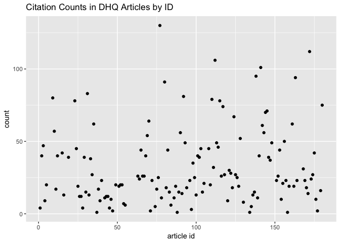
For some context, a plot of the citation counts this looks like this:
citation_count_list %>%
  ggplot() + aes(x = `article id`, y = count) +
  geom_point() +
  ggtitle("Citation Counts in DHQ Articles by ID")
We could group the citation counts instead by publication year to visualize temporal trends in citation within a single article. Does the number of citations used in an article change meaningfully with time?
group_by(citation_counts,`article id`,year) %>%
  summarize(count=n()) %>%
  ggplot() +
  geom_boxplot() +
  aes(x = year, group= year,y = count) +
  ggtitle("Citation Counts in DHQ Articles by Year")
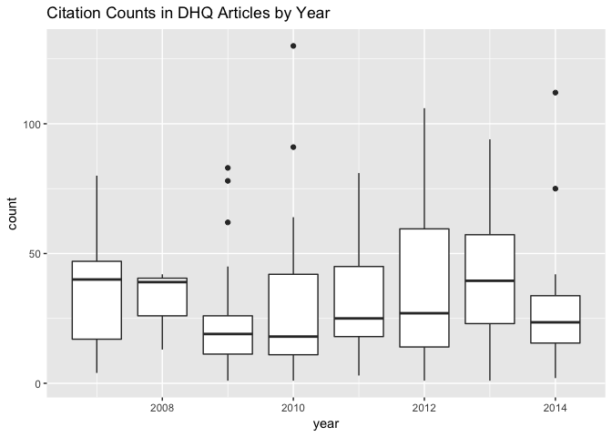
Aggregating the data like this lets us see how statistically out of the ordinary Borgman’s 2010 article is as an outlier.
How many authors do DHQ articles have?
We’ve so far focused on the articles and citations and haven’t said much about the journal’s authors.
The author variables in both tibbles are relatively consistent. Individual author names are listed as “last name, first name” and with a middle initial if applicable; and multiple authors on the same work are separated by pipe characters. Some authors appear to be organizations. Because no local authority control has been implemented, there may well be variation among the author names, which could refer to the same author.
head(dhq_articles$author)
## [1] "Drucker, Johanna" "Howard, Jeff"     "VandeCreek, Drew"
## [4] "Patrik, Linda E." "Wolff, Mark"      "Raben, Joseph"
head(dhq_citations$author)
## [1] "ACTLab"
## [2] "Alliance of Digital Humanities Organizations (ADHO)"
## [3] "Anderson, S."
## [4] "Alliance of Digital Humanities Organizations (ADHO)"
## [5] "annotation-ontology"
## [6] "Agnosti, Maristella | Ferro, Nicola"
By implementing similar code as before that we used to parse and split up the reference IDs, we can parse the authors of each article and display them in a wide tibble.
authors_expanded <- dhq_articles %>%
  mutate(list = strsplit(`author`,"\\|"))  %>%
  unnest(list) %>%
  group_by(`article id`)  %>%
  mutate(row = row_number()) %>%
  spread(row, list)  %>%
  group_by()

authors_expanded %>%
    select(-(author:isDHQ))
## # A tibble: 178 × 16
##    `article id`              `1`             `2`              `3`   `4`
## *         <int>            <chr>           <chr>            <chr> <chr>
## 1             1 Drucker, Johanna            <NA>             <NA>  <NA>
## 2             2     Howard, Jeff            <NA>             <NA>  <NA>
## 3             3 VandeCreek, Drew            <NA>             <NA>  <NA>
## 4             4 Patrik, Linda E.            <NA>             <NA>  <NA>
## 5             5      Wolff, Mark            <NA>             <NA>  <NA>
## 6             6    Raben, Joseph            <NA>             <NA>  <NA>
## 7             7 Flanders, Julia   Piez, Wendell   Terras, Melissa  <NA>
## 8             8    Raben, Joseph            <NA>             <NA>  <NA>
## 9             9  Jerz, Dennis G.            <NA>             <NA>  <NA>
## 10           10        Eve, Eric            <NA>             <NA>  <NA>
## # ... with 168 more rows, and 11 more variables: `5` <chr>, `6` <chr>,
## #   `7` <chr>, `8` <chr>, `9` <chr>, `10` <chr>, `11` <chr>, `12` <chr>,
## #   `13` <chr>, `14` <chr>, `15` <chr>
Now we can, for example, see how many articles have multiple authors.
author_counts <- gather(authors_expanded, "count", "authors", -(`article id`:isDHQ)) %>%
  na.omit()

author_count_list <- group_by(author_counts,`article id`) %>%
  summarize(count=n())

author_count_list %>%
  arrange(desc(count))
## # A tibble: 141 × 2
##    `article id` count
##           <int> <int>
## 1            34    11
## 2            40     6
## 3            43     6
## 4           123     6
## 5            16     5
## 6            44     5
## 7            75     5
## 8            89     5
## 9           111     5
## 10          146     5
## # ... with 131 more rows
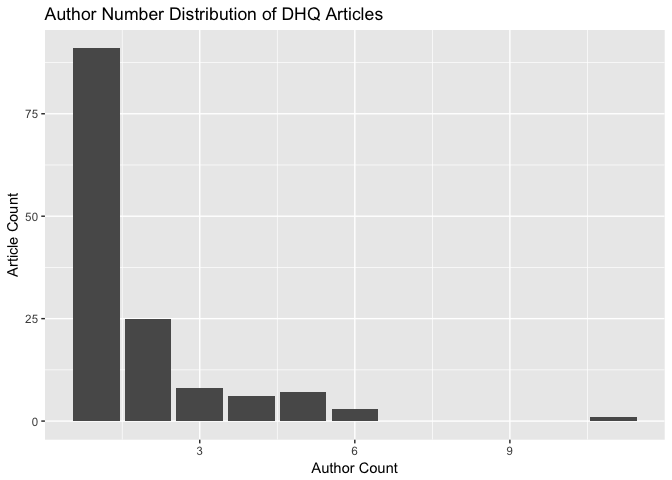
We can get a better look at the number of authors across DHQ articles by plotting a distribution:
author_count_list %>%
  ggplot() + aes(x = count) +
  geom_bar() +
  ggtitle("Author Number Distribution of DHQ Articles") +
    xlab("Author Count") +
  ylab("Article Count")
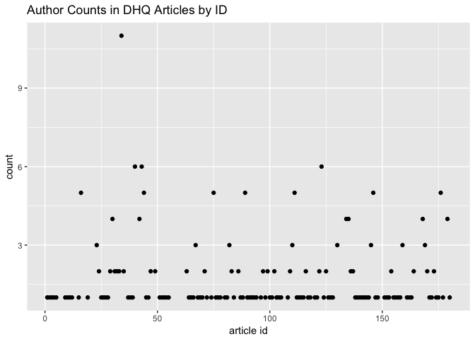
Which articles have the most authors?
author_count_list %>%
  ggplot() + aes(x = `article id`, y = count) +
  geom_point() +
  ggtitle("Author Counts in DHQ Articles by ID")
And when were those highly-collaborative articles published?
group_by(author_counts,`article id`,year) %>%
  summarize(count=n()) %>%
  ggplot() + aes(x = `year`, group=year, y = count) +
  geom_boxplot() +
  ggtitle("Author Counts in DHQ Articles by Year")
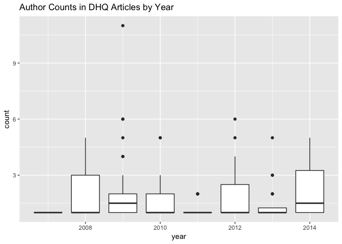
You may have noticed that I’ve elected (neglected?) to interpret these past few plots. Part of this omission is that I’ve sequenced the transformations on this subset of the data, and the plots they yield, to be parallel with another I already performed and described–I intended to aid the reader that way in inferring themselves what could be brought to the plots. Part of the omission is also that I’m running out of steam. But there’s an additional reason. If we take Frederick W. Gibbs’s piece on “Data and Its Representations”” to heart, these visualizations speak for themselves and are not mere augmentations to my written words; conversely, if they are well-formed, they shouldn’t necessarily require alphabetic explanation. I am content with the richness of the box-and-whisker plots to to be self-evident: this is especially since I have no further context to add at this preliminary stage of analysis, the goals of which are to see what questions the data might be able to answer and to get it into a satisfying form. I can’t, for example, offer more information about why Borgman’s 2010 article is a clear outlier in citation count, and it seems silly to reproduce in prose what the plot already communicates solely for the purpose of walking the reader (who I’m assuming knows how to read a box-and-whisker plot) through it to direct their attention to a certain place. In other words, I don’t yet have designs on the data that would provide a compelling rationale for directing that attention.
Still, Grolemund and Wickham acknowledge that exploratory analysis is also about “whether your data meets your expectations or not” (7.1); and I do come to this data with some antecdent knowledge about academic citation that forms the questions I ask. I am feeling the additional tension here, too, of the disciplinary conventions of my physical science background: in the genres of research paper I am used to writing that incorporate visualizations, those visualizations anticipate and are accompanied by narrative text that interprets them according to the experiment’s/study’s research questions–“something that looks like a close reading of experimental results” (Sculley and Pasanek 417). This admission leads to my final suggestion of a research question to bring to the full dataset of encoded articles: how are DHQ authors referencing their charts and figures? What antecedent knowledges do they assume? I’ve also departed from the process-leading “we” to using “I” in some reflective interjections. Accordingly, we could examine with quantiative stylometrics how DHQ authors are using pronouns. Do either of these differ with the article genres and authors’ corresponding disciplinary identities?
Works Cited
Gibbs, Frederick W. “New Forms of History: Critiquing Data and Its Representations.” The American Historian (2016). Web. 23 Jan. 2017.
Grolemund, Garrett, and Hadley Wickham. R for Data Science. r4ds.had.co.nz. Web. 16 Feb. 2017.
Rawson, Katie, and Trevor Muñoz. “Against Cleaning.” (2016). curatingmenus.org. Web. 23 Jan. 2017.
Sculley, D., and Bradley M. Pasanek. “Meaning and Mining: The Impact of Implicit Assumptions in Data Mining for the Humanities.” Literary and Linguistic Computing 23.4 (2008): 409–424. academic-oup-com.ezproxy.neu.edu. Web.